How to Make a Budget in Google Sheets (Free Template, 2026)
By Tapabrata Biswas · Last updated May 10, 2026 · 9 min read
Researched with AI assistance, reviewed and edited by Tapabrata Biswas.

A working Google Sheets budget needs three tabs and four formulas. Total build time from a blank spreadsheet: about 30 minutes. Google Sheets is one of the most popular DIY budgeting tools because it costs nothing, runs in any browser, syncs across devices automatically, and gives the household full control over the structure. The trade-off is that it requires building the budget yourself — there's no app populating categories or syncing transactions automatically.
The good news is that the build is simpler than it looks.
What you'll build
The structure has three sheets.
A Budget tab holds categories, assigned amounts, spent amounts, remaining, and totals. A Transactions tab logs every individual purchase, with date, description, amount, and category. A Summary tab shows month-to-date totals, savings rate, and a simple pie chart.
Most households can run a working budget on just the first tab if they're willing to track spending in aggregate rather than transaction-by-transaction. The second and third tabs are upgrades for households who want more visibility.
Step 1 — open a new Google Sheet and rename it
Go to sheets.google.com, click the blank "+" template, and rename the file something like "Monthly Budget — May 2026." Rename the first tab at the bottom to "Budget."
Step 2 — set up the Budget tab columns
In the first row, type these column headers across columns A through E:
- A1: Category
- B1: Type (essential / variable / savings / discretionary)
- C1: Assigned
- D1: Spent
- E1: Remaining
Bold the row (select row 1, press Ctrl+B / Cmd+B), then freeze it so it stays visible when you scroll: View → Freeze → 1 row.
Step 3 — list your categories
Starting in row 2, list every spending category. A typical 12-category starter list:
| Row | Category | Type |
|---|---|---|
| 2 | Rent | essential |
| 3 | Utilities | essential |
| 4 | Internet | essential |
| 5 | Phone | essential |
| 6 | Insurance | essential |
| 7 | Groceries | variable |
| 8 | Transport | variable |
| 9 | Subscriptions | discretionary |
| 10 | Eating out | discretionary |
| 11 | Personal spending | discretionary |
| 12 | Emergency fund | savings |
| 13 | Retirement | savings |
Fill column A and column B accordingly. Leave columns C, D, and E empty for now.
Step 4 — fill in your assigned amounts
In column C (Assigned), type the amount you want to budget for each category. These are the amounts based on what your income can cover and what you've decided each category should get. For a household earning $4,000 net per month, the row 2 entry might be 1400 for rent, the row 7 entry 480 for groceries, and so on.
The total of all assigned amounts should equal your monthly net income if you're using zero-based budgeting, or roughly fit the 50/30/20 rule's percentages if that's your method.
Step 5 — add the totals row at the bottom
In row 14 (just below your last category), type "TOTAL" in column A. In column C (Assigned total), type this formula:
=SUM(C2:C13)
That tells you the sum of all your assigned amounts. The same formula in column D will sum your spending later: =SUM(D2:D13).
In column E (Remaining), type this formula in each row from row 2 to row 13:
=C2-D2
That calculates how much is left in each category. You can drag the formula down (click cell E2, then drag the blue square in the bottom-right corner down to row 13) so all rows have it.
In E14 (the totals row's "Remaining"), the formula is =C14-D14.
Step 6 — add the Transactions tab
At the bottom of the spreadsheet, click the "+" to add a new tab. Rename it "Transactions." Set up these columns in row 1:
- A1: Date
- B1: Description
- C1: Amount
- D1: Category
Bold and freeze the header row.
As purchases happen during the month, add them as rows here. Date, what it was, how much, and which category. The category should match exactly one of the categories from your Budget tab (so the formula in the next step works).
Step 7 — connect the tabs with SUMIF
Now go back to the Budget tab. Replace the spent amounts (column D) with a formula that automatically sums all transactions in each category from the Transactions tab.
In cell D2, type:
=SUMIF(Transactions!D:D, A2, Transactions!C:C)
That says: "Look in the Category column of the Transactions tab for any row that matches the category in cell A2 of the Budget tab, and sum the corresponding Amount column values."
Drag this formula down from D2 to D13 so every category has it. As you add transactions to the Transactions tab, the Spent column on the Budget tab updates automatically.
Step 8 — add conditional formatting for visual feedback
Conditional formatting highlights overspent categories in red without you having to look closely. Select cells E2:E13 (your Remaining column for the categories), then go to Format → Conditional formatting.
In the panel that opens, set the first rule: Format cells if... Less than... 0. Pick a red background colour. Click "Done."
Add a second rule: Format cells if... Greater than... 0. Pick a green background colour. Click "Done."
Now any category with a negative remaining (overspent) shows red; any category with a positive remaining (room left) shows green. The visual cue makes the weekly check-in faster — overspent categories jump out instantly.
Step 9 — add the Summary tab
Add another tab and name it "Summary." This is for at-a-glance metrics. In cell A1, type "Month-to-date summary." Then build out:
- A3: Total income | B3: [type your net income, e.g. 4000]
- A4: Total spent | B4:
=Budget!D14 - A5: Total remaining | B5:
=B3-B4 - A6: Savings rate | B6:
=SUMIF(Budget!B:B,"savings",Budget!C:C)/B3
In cell B6, format as percentage: select the cell, then Format → Number → Percent.
For a simple pie chart of spending by type: select your Budget tab's Type and Spent columns, then Insert → Chart, choose pie chart. Move the resulting chart to the Summary tab.
Step 10 — set up the weekly update routine
A budget that doesn't get updated isn't a budget. Block 15 minutes once a week to:
- Open your bank's online statement, copy any new transactions
- Paste them as new rows in the Transactions tab (Date, Description, Amount, Category)
- Glance at the Budget tab — any red cells need attention
- If a category is on track to overspend, decide whether to cut spending there or move money from another category that has surplus
The total at the bottom of the Budget tab should still equal your monthly income at all times. Moving money between categories changes individual amounts but not the total.
Optional upgrades
Several upgrades extend the basic build for households who want more.
Multi-month tracking is the simplest: duplicate the Budget tab each month (rename "Budget May 2026," "Budget June 2026," etc.) so you can see how categories change over time.
Sparklines add visual context. In a row at the bottom, use =SPARKLINE(...) to show small inline trend charts of spending per category over multiple months.
Tiller Money integration removes the manual paste step entirely. Tiller Money is a paid service ($79/year) that automatically pulls bank transactions into a Google Sheet daily. Worth it for households who find the manual update friction is what kills their consistency.
An income tab helps if your income varies. Add a third tab to track each paycheck or invoice, with the total feeding into the Summary tab's "Total income" cell.
Common mistakes when building a Sheets budget
Four patterns trip people up regularly when they build a Sheets budget.
The first is not freezing the header rows. The first scroll down loses the column labels and makes everything harder to read.
The second is typo'd category names. SUMIF requires exact text matches. "Eating out" in the Budget tab and "eating out" in the Transactions tab won't match (capitalisation matters in some Sheets configurations).
The third is no totals row. Without =SUM(C2:C13) and =SUM(D2:D13), you can't see whether the budget balances.
The fourth is overengineering before using it. A six-tab spreadsheet with macros, dashboards, and conditional formatting takes hours to build and gets abandoned because the maintenance is overwhelming. Start simple; expand only if a specific feature would save more time than it costs.
What experts say
NerdWallet's spreadsheet budget guide covers similar ground with screenshots and formula examples. Investopedia's coverage of personal finance spreadsheets compares spreadsheet budgeting against app-based alternatives.
For a printable version of the same structure that doesn't require Google Sheets, see our monthly budget template. For the underlying budgeting framework choices that determine which categories and amounts to put into your sheet, see how to make a budget.
Frequently asked questions
Why use Google Sheets instead of a budgeting app? Google Sheets is free, doesn't require granting bank-account access to a third party, and gives full control over the formulas and layout. The trade-off is manual data entry — apps like YNAB or Monarch sync transactions automatically, while a Sheets budget needs you to type or paste in transactions yourself. For households who prefer privacy and customisation over convenience, Sheets is the standard choice.
What are the most important formulas in a Google Sheets budget? Three formulas cover 90% of what a budget needs: SUMIF (to sum spending by category), SUM (to total a column), and a simple subtraction (assigned minus spent = remaining). For more advanced budgets, SPARKLINE (small inline charts) and conditional formatting (highlighting overspent categories) add real value without much complexity.
Can I import my bank transactions into Google Sheets? Most banks let you download transactions as a CSV file, which Google Sheets opens directly. Some banks offer "OFX" format which also works. For automated syncing, Tiller Money is a paid service ($79/year as of 2026) that connects bank accounts to a Google Sheet daily. Without Tiller, expect to download and paste transactions manually once or twice a month.
How long does it take to set up a Google Sheets budget? About 30–45 minutes for a simple monthly budget with categories and formulas. Add another 30 minutes if you want conditional formatting, charts, or a transactions tab. Templates from sites like Vertex42 or Tiller's free template library can reduce the build time to 5–10 minutes if you don't want to build from scratch.
How do I create a budget in Google Sheets step by step? Open a new sheet and rename the first tab Budget. Add columns for Category, Type, Assigned, Spent, and Remaining, then list your spending categories down column A. Put the planned amount for each in the Assigned column, use =SUM() for a totals row, and =C2-D2 for what's left in each category. Add a Transactions tab to log purchases, then connect the two with =SUMIF(Transactions!D:D, A2, Transactions!C:C) so the Spent column updates itself. That gives you a working budget in about 30 minutes, and the full build is the 10 steps in this guide.
Do I need a template, or can I build a Google Sheets budget from scratch? You can build one from scratch in about 30 minutes, and this guide walks through it step by step. The only formulas you need are SUM for column totals, SUMIF for spending by category, and a subtraction for what's remaining. If you'd rather start from a pre-built layout, the Google Sheets template gallery includes a Monthly budget and an Annual budget template, and sites like Vertex42 offer free versions you copy to your own Drive.
In summary
A working Google Sheets budget needs three tabs (Budget, Transactions, Summary), a handful of formulas (SUMIF for category totals, SUM for column totals, a subtraction for remaining), and a weekly routine to update transactions. The build takes 30–45 minutes from scratch. The advantages over apps are cost (free), privacy (no third-party bank access), and flexibility (any formula or layout you want); the trade-off is manual transaction entry.
The single feature that distinguishes a Sheets budget that gets used from one that gets abandoned isn't the formulas or the conditional formatting. It's the recurring 15-minute weekly slot on the calendar to paste in transactions. Without that habit, even the most beautifully-formulated spreadsheet sits stale by week three.
The spreadsheet is just the tool; for the framework that goes inside it, you can compare the main budgeting methods.
Sources
- NerdWallet, Spreadsheet Budgeting Tips — nerdwallet.com/article/finance/budget-spreadsheet-tips
- Investopedia, Personal Finance Spreadsheets and Apps — investopedia.com/articles/personal-finance/061216/best-budgeting-apps-software-2016.asp
- Tiller Money — tillerhq.com
- Google Sheets — sheets.google.com
Continue reading — more from Budgeting
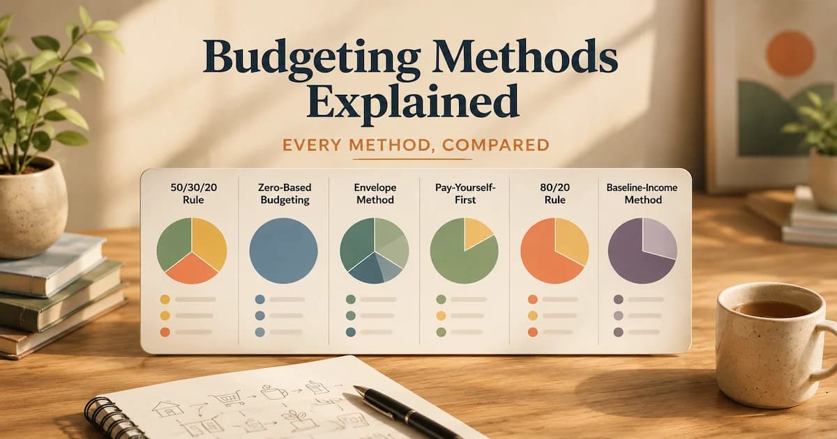
Every personal budgeting method compared side by side, with worked examples in ₹ and $, a guide to which method fits you, and an honest note on where each one fails.
13 min read

Why budgeting is important — the research findings on financial well-being, the structural reasons budgets work even when willpower doesn't, and the long-term costs of not having one.
9 min read

What is zero-based budgeting? A plain-English definition, how the method works step by step, a worked example, and the misconceptions that trip up beginners.
9 min read